These Excel spill formulas make dynamic dashboards ridiculously easy

2025 October 29 • AI Tools

These Excel Spill Formulas Make Dynamic Dashboards Ridiculously Easy

SEO Meta Description

Discover how Excel’s dynamic array functions like UNIQUE, FILTER, BYROW, REDUCE, and SCAN can transform your dashboards into self-updating powerhouses. Learn setup, use cases, and comparisons with alternatives.

Introduction

For years, building dashboards in Excel meant juggling helper columns, dragging formulas across endless cells, and praying your pivot table wouldn’t collapse under its own weight. But that’s changed. With the arrival of dynamic arrays, Excel has introduced a smarter, cleaner way to work: spill formulas.

Using just one formula, you can create an entire table, generate a filtered view, calculate a running total, or build a compact list that updates itself every time your data changes. If you’re ready to let Excel do the heavy lifting while you focus on insights, these might be the functions you didn’t know you needed.

Overview of Spill Formulas

Spill formulas in Excel dynamically adjust their output range based on the size of the data they process. Unlike traditional formulas that require manual expansion, spill formulas automatically “spill” their results into adjacent cells, making them ideal for dynamic dashboards. These functions are available in Excel for Microsoft 365, Excel for Microsoft 365 for Mac, or Excel for the web. Some may also be available in Excel 2021 or Excel 2024, but availability varies.

Key Spill Formulas and Their Benefits

1. UNIQUE: The Smart Way to Build Dynamic Lists

Overview:
The UNIQUE function returns a list of distinct values from a range or array. It’s perfect for pulling product names, departments, months, or any other category from your source data. As your dataset updates, the extracted list refreshes automatically.

Syntax:

=UNIQUE(array, [by_col], [exactly_once])

Key Features:

Dynamic Lists: Automatically updates when new data is added.
Customizable Output: Sort results alphabetically or numerically by wrapping with SORT.
Flexible Filtering: Use exactly_once to return only values that appear once.

Use Case:
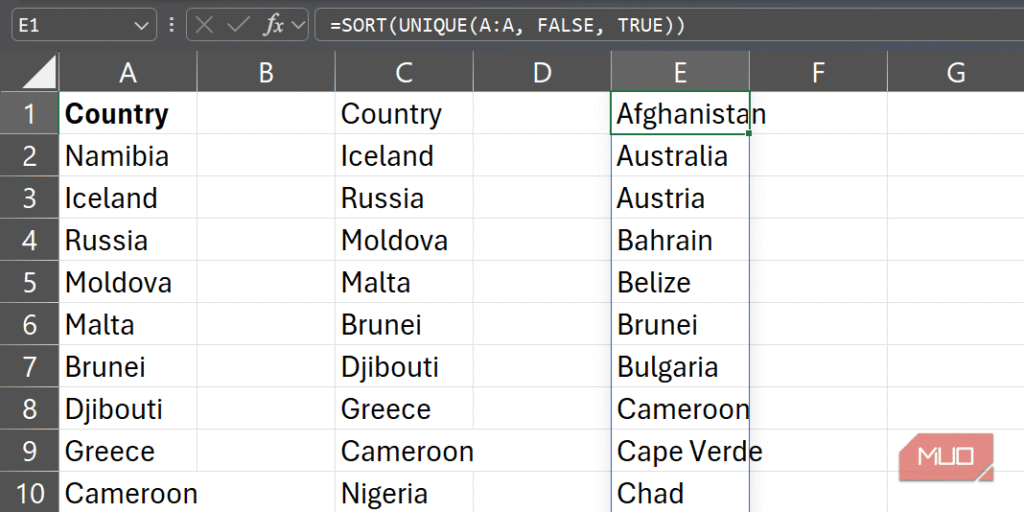
Imagine you have a list of product names in column A, imported from a form where entries often repeat. With UNIQUE, you can instantly transform that messy list into a clean dropdown source or slicer that updates as new values arrive:

=UNIQUE(A:A, FALSE, TRUE)

To display the list in alphabetical order:

=SORT(UNIQUE(A:A, FALSE, TRUE))

Business Application:

Sales Dashboards: Create dynamic dropdowns for product categories.
HR Reports: Generate lists of unique employee departments or roles.

2. FILTER: Instant, Auto-Updating Data Views

Overview:
The FILTER function applies one or more criteria to a range and returns only the rows that meet your conditions. It’s ideal for answering conditional questions like, “Show me only the high-value deals” or “What are my Q4 revenue figures?”

Syntax:

=FILTER(array, include, [if_empty])

Key Features:

Conditional Filtering: Apply single or multiple criteria.
Dynamic Updates: Automatically refreshes when source data changes.
Custom Messages: Use if_empty to display a message when no results are found.

Use Case:
To filter rows where the Sales Channel column (column D) equals “Online”:

=FILTER(A2:N100, D2:D100="Online", "")

To make it easier to change the filter, reference a cell with the condition:

=FILTER(A2:N100, D2:D100=O2, "")

Combine with SORT to arrange results alphabetically or numerically:

=SORT(FILTER(A2:N100, (D2:D100=O2)*(I2:I100>1500)))

Business Application:

Financial Reports: Filter transactions by date, amount, or category.
Inventory Management: Show only out-of-stock items.

3. BYROW: Smarter Calculations Per Row Without Helper Columns

Overview:
The BYROW function applies a LAMBDA function to each row of a specified array and returns the results as a vertical spill. It’s perfect for performing row-specific calculations without altering your original data.

Syntax:

=BYROW(array, lambda(row))

Key Features:

Row-Specific Calculations: Perform unique calculations for each row.
No Helper Columns: Eliminates the need for additional columns.
Flexible Logic: Use LAMBDA to define custom calculations.

Use Case:
To find the highest value in each row:

=BYROW(AM2:AR100, LAMBDA(r, MAX(r)))

To calculate a per-row margin by subtracting unit cost from unit price:

=BYROW(AN2:AO100, LAMBDA(r, INDEX(r, 1, 1) - INDEX(r, 1, 2)))

Business Application:

Sales Analysis: Calculate margins or discounts per transaction.
Project Management: Track task completion rates row by row.

4. REDUCE: Summaries That Adapt Automatically

Overview:
The REDUCE function condenses an entire array into a single accumulated result by repeatedly applying a LAMBDA function to each value. It’s ideal for complex summaries that evolve with your data.

Syntax:

=REDUCE([initial_value], array, lambda(accumulator, value, body))

Key Features:

Accumulated Results: Condenses data into a single value.
Complex Logic: Apply multiple rules or nested conditions.
Dynamic Updates: Automatically adjusts as your dataset changes.

Use Case:
To sum only values exceeding 100,000:

=REDUCE(0, AP2:AP100, LAMBDA(total,value, IF(value>100000, total+value, total)))

Business Application:

Financial Summaries: Calculate total high-value transactions.
Inventory Management: Compute cumulative stock levels.

5. SCAN: See Change Happen Over Time

Overview:
The SCAN function returns all intermediate results of an accumulation process, unlike REDUCE, which only returns the final result. It’s perfect for visualizing trends and progress over time.

Syntax:

=SCAN([initial_value], array, lambda(accumulator, value, body))

Key Features:

Intermediate Results: Shows the journey to the final result.
Trend Analysis: Ideal for rolling forecasts or progressive dashboards.
Dynamic Visualization: Feed results into charts for real-time updates.

Use Case:
To track the accumulation of values exceeding 100,000:

=SCAN(0, AP2:AP100, LAMBDA(total,value, IF(value>100000, total+value, total)))

Business Application:

Sales Tracking: Visualize revenue growth over time.
Project Management: Monitor task completion progress.

Setup Process and Cost

Requirements:

Excel for Microsoft 365 (Windows or Mac)
Excel for the web (limited functionality)
Excel 2021 or Excel 2024 (partial support)

Cost:

Microsoft 365 Subscription: Starts at $6.99/month for personal use.
One-Time Purchase: Excel 2021 or Excel 2024 (check current pricing).

Comparison with Alternatives

Feature	Spill Formulas (Excel)	Traditional Excel Methods	Power BI	Tableau
Dynamic Updates	✅ Yes	❌ Manual updates	✅ Yes	✅ Yes
Ease of Use	✅ Beginner-friendly	❌ Complex	⚠️ Learning curve	⚠️ Learning curve
Cost	✅ Affordable	✅ Free (with Excel)	❌ Subscription	❌ Subscription
Customization	✅ High	⚠️ Limited	✅ High	✅ High
Integration	✅ Seamless	✅ Native	✅ Cloud-based	✅ Cloud-based

Conclusion

Excel’s spill formulas like UNIQUE, FILTER, BYROW, REDUCE, and SCAN are game-changers for dynamic dashboards. They eliminate the need for manual updates, reduce errors, and save time, allowing you to focus on insights rather than maintenance. Whether you’re managing sales data, financial reports, or project tracking, these functions can transform your workflow.

Ready to streamline your dashboards? Start experimenting with these spill formulas today and experience the power of dynamic, self-updating Excel dashboards!

Tags: AI Automation Tools